
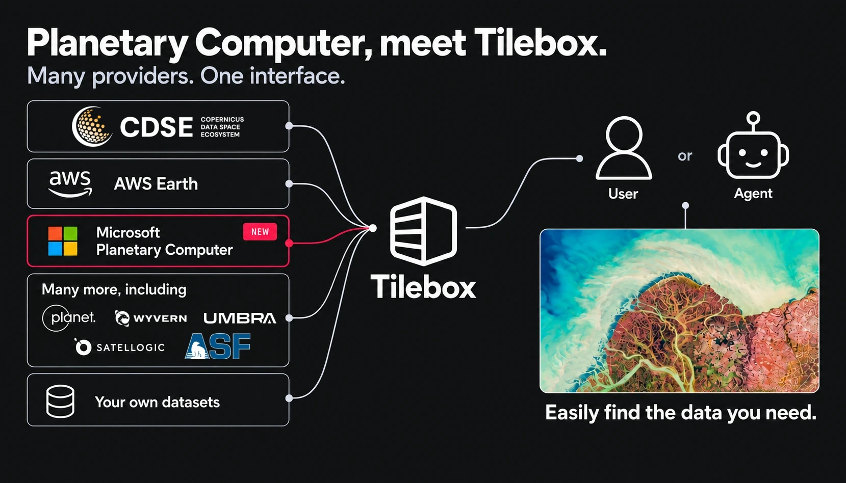
We’ve added new open data datasets from Microsoft Planetary Computer to Tilebox. We’re starting with Landsat, MODIS, and Sentinel-5P, and you can use them alongside other providers and your own datasets.
The new storage-client integration lets you open the files directly from a query result. You don’t need an API key, a separate provider account, or requester-pays setup. Tilebox handles Planetary Computer’s temporary access tokens.
Here’s what you can work with:
- Landsat: imagery going back to 1972, plus surface reflectance and temperature data. Use it to study how cities, farmland, and ecosystems have changed over decades.
- MODIS: vegetation indices, land-surface temperature, and surface reflectance. Useful for following seasonal changes across large areas.
- Sentinel-5P: measurements of gases such as nitrogen dioxide and methane, plus aerosols and clouds, for studying the atmosphere and air quality.
They’re available as open_data.planetary_computer.landsat, open_data.planetary_computer.modis, and open_data.planetary_computer.sentinel5p.
Landsat and MODIS offer Cloud Optimized GeoTIFFs (COGs), so you can read a small area without downloading a whole scene. Sentinel-5P comes in NetCDF format.
This notebook example finds a Landsat scene with less than 5% cloud cover and reads its red, green, and blue bands over the Exuma islands in the Bahamas:
import asyncio

from shapely import box
from tilebox.datasets import Client, field
from tilebox.datasets.assets import AssetCollection
from tilebox.storage.aio import Client as StorageClient
from tilebox.storage.geotiff import window_from_bounds

area = box(-76.8, 24.10, -76.3, 24.45)  # Exuma, Bahamas
landsat = Client().dataset("open_data.planetary_computer.landsat")
scenes = landsat.collection("L2").query(
    temporal_extent=("2024-01-01", "2024-01-02"),
    spatial_extent=area,
    filter=field("cloud_cover") < 5,
)
assets = AssetCollection.from_datapoint(
    scenes.sortby("cloud_cover").isel(time=0)
)

storage = StorageClient()

async def read_band(band):
    cog = await storage.open_geotiff(assets[band])
    window = window_from_bounds(cog, area.bounds, crs="EPSG:4326")
    return await cog.read(window=window)

# fetch in parallel
red, green, blue = await asyncio.gather(
    read_band("red"), read_band("green"), read_band("blue")
)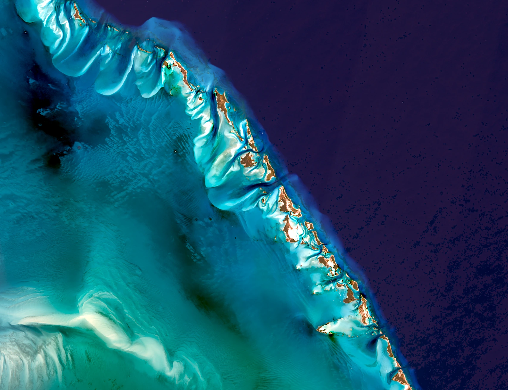
The code returns raw pixel values. For the image above, we applied the bands’ scale and offset and the display settings from our RGB guide. Use the product’s quality masks for analysis.
See how to open files and read a region with the storage client.