In just five lines of Python, you can query every Sentinel-2 scene over any location on Earth – filtered by time, geography, and cloud cover — with the Tilebox Open Data catalog.
No ESA account, no Copernicus API credentials, no OAuth dance required. Install one package, point it at the Tilebox Open Data catalog, and get an xarray Dataset back.
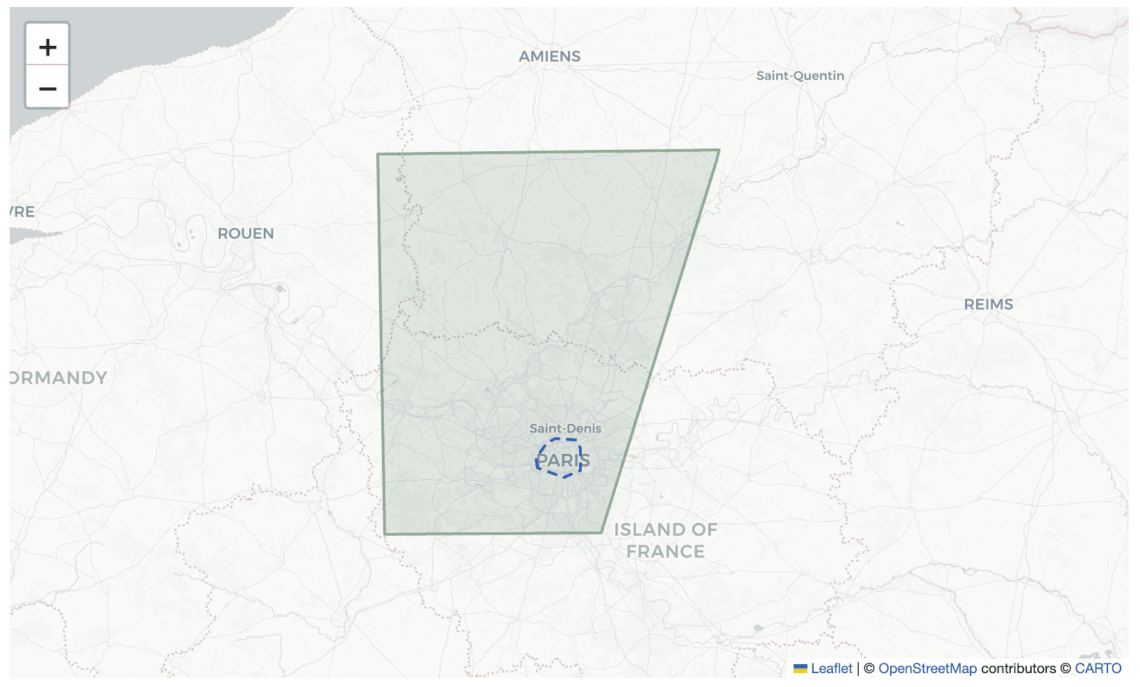
The output is an interactive folium map showing Sentinel-2 scene footprints over your area of interest, colored by cloud cover percentage. Open in Google Colab here.
Install Tilebox
That's the only dependency you need for querying. We'll add folium and matplotlib later for visualization.
Query Sentinel-2 scenes over a location
Pick a location and a time range. This example queries all Sentinel-2 Level 2A scenes over Paris during September 2025.
from shapely import Polygon
from tilebox.datasets import Client

# Polygon around Paris
paris = Polygon([
    (2.245958, 48.8311913), (2.2436426, 48.8577043),
    (2.2843926, 48.896382), (2.3172704, 48.9088622),
    (2.4006226, 48.9055141), (2.4186822, 48.8829853),
    (2.4182191, 48.8238749), (2.3520005, 48.8058842),
    (2.245958, 48.8311913),
])

client = Client()
dataset = client.dataset("open_data.copernicus.sentinel2_msi")
data = dataset.query(
    collections=["S2A_S2MSI2A", "S2B_S2MSI2A", "S2C_S2MSI2A"]
No API key required. The Client() constructor connects to the Tilebox open data catalog by default when querying public datasets. The dataset.query() call queries across all three Sentinel-2 satellites (2A, 2B, 2C) and returns the results as an xarray.Dataset.
The spatial extent here is a polygon around central Paris, but it accepts any Polygon or MultiPolygon — country outlines, watersheds, coastlines, or any arbitrary shape you can define with Shapely. Tilebox also handles antimeridian crossings and pole-covering geometries correctly out of the box.
<xarray.Dataset> Size: 19kB
Dimensions:                (time: 42)
Coordinates:
  * time                   (time) datetime64[ns]
<xarray.Dataset> Size: 19kB
Dimensions:                (time: 42)
Coordinates:
  * time                   (time) datetime64[ns]
<xarray.Dataset> Size: 19kB
Dimensions:                (time: 42)
Coordinates:
  * time                   (time) datetime64[ns]
Each row is one Sentinel-2 scene. The dataset includes the scene geometry, cloud cover percentage, thumbnail URL, granule name, and 20+ other metadata fields — all indexed by acquisition time.
Explore the results with xarray
The output is a standard xarray Dataset. You can filter, slice, and analyze it with any operation xarray supports.
Check how many scenes were acquired and what the cloud cover distribution looks like:
print(f"Found {data.sizes['time']
print(f"Found {data.sizes['time']
print(f"Found {data.sizes['time']
Filter by cloud cover
Most workflows start with filtering out cloudy scenes. xarray makes this straightforward:
clear_scenes = data.where(data.cloud_cover < 20, drop=True)
print(f"{clear_scenes.sizes['time']
clear_scenes = data.where(data.cloud_cover < 20, drop=True)
print(f"{clear_scenes.sizes['time']
clear_scenes = data.where(data.cloud_cover < 20, drop=True)
print(f"{clear_scenes.sizes['time']
You can also sort by cloud cover to find the clearest acquisitions:
import numpy as np

sorted_indices = np.argsort(data.cloud_cover.values)
clearest = data.isel(time=sorted_indices[:5])
for i in range(clearest.sizes['time']
import numpy as np

sorted_indices = np.argsort(data.cloud_cover.values)
clearest = data.isel(time=sorted_indices[:5])
for i in range(clearest.sizes['time']
import numpy as np

sorted_indices = np.argsort(data.cloud_cover.values)
clearest = data.isel(time=sorted_indices[:5])
for i in range(clearest.sizes['time']
Plot scene footprints on an interactive map
Install the visualization dependencies:
Now plot every scene footprint on a folium map, colored by cloud cover percentage. Green means clear skies, red means heavy cloud cover.
import folium
import matplotlib
import matplotlib.cm as cm

# Create a map centered on our area of interest
center_lat = (52.3 + 52.7) / 2
center_lon = (13.1 + 13.8) / 2
m = folium.Map(location=[center_lat, center_lon], zoom_start=10)

# Color scale: green (clear) to red (cloudy)
norm = matplotlib.colors.Normalize(vmin=0, vmax=100)
colormap = cm.RdYlGn_r

for i in range(data.sizes['time']):
    scene = data.isel(time=i)
    cloud = scene.cloud_cover.item()
    rgba = colormap(norm(cloud))
    color = matplotlib.colors.to_hex(rgba)

    # Extract polygon coordinates from the geometry
    geom = scene.geometry.item()
    coords = [(lat, lon) for lon, lat in geom.exterior.coords]

    folium.Polygon(
        locations=coords,
        color=color,
        fill=True,
        fill_color=color,
        fill_opacity=0.4,
        popup=f"{scene.time.dt.strftime('%Y-%m-%d').item()}<br>"
              f"Cloud cover: {cloud:.1f}%<br>"
              f"{scene.granule_name.item()}",
    ).add_to(m)

# Add a bounding box for the area of interest
folium.Rectangle(
    bounds=[(52.3, 13.1), (52.7, 13.8)]
Open the map in a Jupyter notebook and click on any footprint to see the acquisition date, cloud cover, and granule name.
Scene footprint
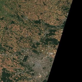
Preview a scene thumbnail
Each Sentinel-2 scene in the Tilebox catalog includes a thumbnail URL. You can display it directly in a notebook:
from IPython.display import Image, display

# Pick the clearest scene
sorted_indices = np.argsort(data.cloud_cover.values)
best_scene = data.isel(time=sorted_indices[0]
from IPython.display import Image, display

# Pick the clearest scene
sorted_indices = np.argsort(data.cloud_cover.values)
best_scene = data.isel(time=sorted_indices[0]
from IPython.display import Image, display

# Pick the clearest scene
sorted_indices = np.argsort(data.cloud_cover.values)
best_scene = data.isel(time=sorted_indices[0]
Scene thumbnail
What you just did
In under 30 lines of code, you:
Connected to Tilebox's open data catalog — no API key, no account
Queried all Sentinel-2 Level 2A scenes over Paris for a full month
Filtered scenes by cloud cover using standard xarray operations
Plotted every scene footprint on an interactive map, color-coded by cloud cover
Previewed a scene thumbnail
The query returned structured metadata as an xarray Dataset: scene geometries, acquisition timestamps, cloud cover percentages, thumbnail URLs, and granule identifiers. From here you can feed the results into any processing pipeline, download the actual data from Copernicus Data Space, or build automated monitoring workflows with Tilebox.
Downloading the actual scene data
Tilebox indexes satellite metadata — the full scene data (bands, reflectance values) lives in the Copernicus Data Space Ecosystem. Once you've identified the scenes you want, you can download them using the Tilebox storage client:
from tilebox.storage import CopernicusStorageClient

storage_client = CopernicusStorageClient(
    access_key="YOUR_CDSE_ACCESS_KEY",
    secret_access_key="YOUR_CDSE_SECRET_KEY",
)

for i in range(clear_scenes.sizes['time']
from tilebox.storage import CopernicusStorageClient

storage_client = CopernicusStorageClient(
    access_key="YOUR_CDSE_ACCESS_KEY",
    secret_access_key="YOUR_CDSE_SECRET_KEY",
)

for i in range(clear_scenes.sizes['time']
from tilebox.storage import CopernicusStorageClient

storage_client = CopernicusStorageClient(
    access_key="YOUR_CDSE_ACCESS_KEY",
    secret_access_key="YOUR_CDSE_SECRET_KEY",
)

for i in range(clear_scenes.sizes['time']
This requires free Copernicus Data Space credentials — but querying and filtering metadata through Tilebox is completely open.
Full script
Here's the complete script in one block. Copy it into a Jupyter notebook or Python file and run it top to bottom.
from shapely import Polygon
from tilebox.datasets import Client
import numpy as np
import folium
import matplotlib
import matplotlib.cm as cm
from IPython.display import Image, display

# 1. Define your area of interest
berlin = Polygon((
    (13.1, 52.3),
    (13.1, 52.7),
    (13.8, 52.7),
    (13.8, 52.3),
    (13.1, 52.3),
))

# 2. Query Sentinel-2 scenes (no API key needed)
client = Client()
dataset = client.dataset("open_data.copernicus.sentinel2_msi")
data = dataset.query(
    collections=["S2A_S2MSI2A", "S2B_S2MSI2A", "S2C_S2MSI2A"],
    temporal_extent=("2025-09-01", "2025-10-01"),
    spatial_extent=berlin,
    show_progress=True,
)

# 3. Print summary
print(f"Found {data.sizes['time']} Sentinel-2 scenes")
print(f"Cloud cover: min={data.cloud_cover.min().item():.1f}%, "
      f"max={data.cloud_cover.max().item():.1f}%, "
      f"mean={data.cloud_cover.mean().item():.1f}%")

# 4. Filter by cloud cover
clear_scenes = data.where(data.cloud_cover < 20, drop=True)
print(f"{clear_scenes.sizes['time']} scenes with less than 20% cloud cover")

# 5. Plot footprints on an interactive map
center_lat = (52.3 + 52.7) / 2
center_lon = (13.1 + 13.8) / 2
m = folium.Map(location=[center_lat, center_lon], zoom_start=10)

norm = matplotlib.colors.Normalize(vmin=0, vmax=100)
colormap = cm.RdYlGn_r

for i in range(data.sizes['time']):
    scene = data.isel(time=i)
    cloud = scene.cloud_cover.item()
    rgba = colormap(norm(cloud))
    color = matplotlib.colors.to_hex(rgba)
    geom = scene.geometry.item()
    coords = [(lat, lon) for lon, lat in geom.exterior.coords]

    folium.Polygon(
        locations=coords,
        color=color,
        fill=True,
        fill_color=color,
        fill_opacity=0.4,
        popup=f"{scene.time.dt.strftime('%Y-%m-%d').item()}<br>"
              f"Cloud cover: {cloud:.1f}%<br>"
              f"{scene.granule_name.item()}",
    ).add_to(m)

folium.Rectangle(
    bounds=[(52.3, 13.1), (52.7, 13.8)],
    color="blue",
    fill=False,
    weight=2,
).add_to(m)

m

# Display the map in a Jupyter notebook

# 6. Preview the clearest scene thumbnail
sorted_indices = np.argsort(data.cloud_cover.values)
best_scene = data.isel(time=sorted_indices[0]
Next steps
To run this yourself, install Tilebox with uv add tilebox (or pip install tilebox) and open the full notebook from the tilebox/examples repository. Swap out the Paris polygon for your own coordinates and you'll have a map of your area's Sentinel-2 coverage in under five minutes.